Logistics
You can download the raw material from KLMS.
To do
-
Code template in
code/. -
Writeup template in
writeup/.
Submission
|
QnA
-
We will update FAQ on Notice board of KLMS.
-
Before asking a question, please check whether your question is already answered in the FAQ.
-
Please use KLMS QnA board, and title of the post like: [hw5] question about … .
-
Please post the question as opened and english since other student may have same question.
-
Note that TAs are trying to answer question ASAP, but it may take 1—2 day on weekend. Please post the question on weekday if possible.
-
TA in charge: Jiwoong Na <jwna1885@kaist.ac.kr>
Overview
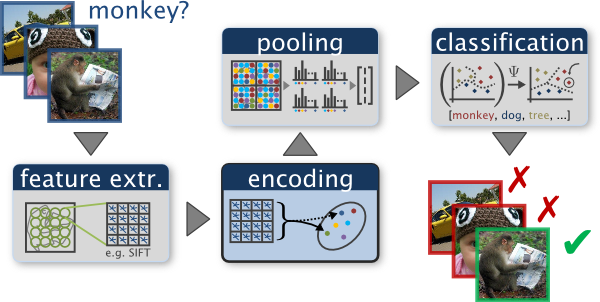
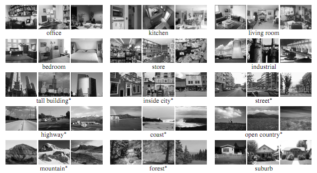
We will perform scene recognition with the bag of words method. We will classify scenes into one of 15 categories by training and testing on the 15 scene database (Lazebnik et al. 2006).
Task: Implement scene recognition schemes:
-
(a) Build vocabulary by k-means clustering (
feature_extraction.py). -
(b) Principle component analysis (PCA) for vocabulary (
get_features_from_pca.py). -
(c) Bag of words representation of scenes (
get_bags_of_words.py, get_spatial_pyramid_feats.py) -
(d) Multi-class SVM (
svm_classify.py).
Forbidden functions
-
sklearn.decomposition.PCA() -
Any other pre-implemented functions to get direct result of main task.
Useful functions
-
cv2.imread(), cv2.HOGDescriptor(), cv2.SIFT_create(), cv2.kmeans(), cv2.KeyPoint_convert()fromopencv-python. -
numpy.meshgrid(), numpy.stack(), numpy.sort(), numpy.argsort(), numpy.concatenate(), numpy.squeeze(), numpy.cov(), numpy.linalg.eig(), numpy.einsum()fromnumpy. -
svm.SVC(), svm.LinearSVC(), svm.SVC.fit(), svm.SVC.decision_function()fromscikit-learn.
Important note about svm.SVC()
-
You should set the
decision_function_shapeto 'ovo'. -
svm.SVC(… , decision_function_shape='ovo', …). -
If you use
svm.SVC()without setting this parameter, you will get 0 points for the corresponding part.
Code details
Main function: The starter code function main.py runs the entire recognition process. You do not have to modify main.py, but you can fill your code in several other files which is called by the main() function.
Data: The starter codes trains and tests on 100 images from each category (i.e. 1500 training examples total and 1500 test cases total). In a real research paper, one would be expected to test performance on random splits of the data into training and test sets, but the starter code does not do this to ease debugging.
Evaluation and Visualization: The starter code function create_results_webpage.py builds a confusion matrix and visualizes your classification decisions by producing a table of true positives, false positives, and false negatives as a webpage.
You can modify only the parts of the source code commented "Your code here". [NB] Do not modify any other parts.
You CANNOT modify following starter codes:
-
main.py -
get_image_paths.py -
build_vocabulary.py -
pca_visualize.py -
distance.py -
create_results_webpage.py
You should fill your code in following files:
-
feature_extraction.py -
get_features_from_pca.py -
get_bags_of_words.py -
get_spatial_pyramid_feats.py -
svm_classify.py
Task details and notes
Lazebnik et al. 2006 is a great paper to read. For an excellent survey of modern feature encoding methods for bag of words models, please see Chatfield et al. 2011..
Build vocabulary by k-means clustering
(a) Feature extraction
-
Fix:
feature_extraction.py
Bag of words models are a popular technique for image classification inspired by models used in natural language processing. The model ignores or downplays word arrangement (spatial information in the image) and classifies based on a histogram of the frequency of visual words. The visual word "vocabulary" is established by clustering a large corpus of local features. See Szeliski chapter 14.4.1 [1st ed.] / 6.2.1 [2nd ed.] for more details on category recognition with quantized features. In addition, 14.1 [1st ed.] / 6.3 [2nd ed.] covers classification techniques.
Strat by extracting features from training data images. We can use cv2 Python library functions cv2.SIFT_create() and cv2.HOGDescriptor() to scale-invariant feature transform (SIFT) features and histogram of oriented gradients (HOG) features, respectively. You should implement to extract features using both of these in feature_extraction.py. You can use cv2 library functions for SIFT and HOG feature extractors, but you should investigate how to use these functions and convert their returns into desired format, suggested by comment lines in feature_extraction.py. Note that we have learned that there are two ways regular grid and interest regions for feature extraction in the lecture (see p.61 in slide22). In this homework you should implement via regular grid. When you implement SIFT, use an image grid size 20, and use an image grid size 16 for HOG. If we run SIFT feature extractor with parameters given in the starter code then the feature dimension becomes 128, and if we run HOG then it becomes 36.
k-means clustering
After we have implemented a baseline scene recognition pipeline, we shall move on to a more sophisticated image representation: bags of quantized feature descriptors. Before we can represent our training and testing images as bags of feature descriptors, we first need to establish a vocabulary of visual words, which will represent the similar local regions across the images in our training database. We will form this vocabulary by clustering with k-means the many thousands of local feature vectors from our training set.
You do not need to implement k-means algorithm by yourself. Instead, you can use cv2.kmeans function call written in build_vocabulary.py line 32 as it is.
Note: This is not the same as finding the k-nearest neighbor feature descriptors! For example, given the training database, we might start by clustering our local feature vectors into k=50 clusters. The centroids of these clusters are our visual word vocabulary. For any new feature point we observe, we can find the nearest cluster to know its visual word. As it can be slow to sample and cluster many local features, the starter code saves the cluster centroids and avoids recomputing them on future runs. Be careful of this if you re-run with different parameters. See Lines 55-63 in main.py for more details.
(b) Principle component analysis (PCA) for vocabulary
-
Fix:
get_features_from_pca.py
We will not apply PCA for the final result of scene recognition in this assignment, but PCA is a significant technique of data analysis. You should implement PCA on our vocabulary, a set of feature vectors, and reduce the feature dimension to 3. The implemented code should be written into get_features_from_pca.py, and you should visualize the PCA result using the starter code pca_visualize.py. Attach the visualization figure to your writeup document.
(c) Bag of words representation of scenes
-
Fix:
get_bags_of_words.py
Now we are ready to represent our training and testing images as histograms of visual words. For each image we will densely sample many feature descriptors. Instead of storing hundreds of feature descriptors, we simply count how many feature descriptors fall into each cluster in our visual word vocabulary. This is done by finding the nearest neighbor k-means centroid for every feature descriptor. Thus, if we have a vocabulary of 50 visual words, and we detect 220 features in an image, then our bag of words representation will be a histogram of 50 dimensions where each bin counts how many times a feature descriptor was assigned to that cluster and sums to 220. The histogram should be normalized using L2-norm so that the image size and the number of features do not dramatically change the bag of feature magnitude. You should implement code to get bag of words representation as a histogram from given image file in get_bags_of_words.py. The starter code function pdist() in distance.py may be helpful to get distances between the feature vector and each of vocabularies.
Spatial pyramid representation
-
Fix:
get_spatial_pyramid_feats.py
A histogram of an image does not tell anything about spatial information. Thus, there is an extended version of histograms with little more spatial information. We will represent the bag of words using spatial pyramids. For each level \$l\$ of the spatial pyramids, the image is divided into \$4^l\$ subimages. For example, if we have the maximum level \$l_{max}=2\$ then there are total \$1+4+16=21\$ subimages. You should implement histograms of each subimages. Let \$h_{ij}\$ (\$i=0,\cdots,l_{max}\$, \$j=1,\cdots,4^i\$) denote the histogram vector of the \$j\$-th subimage in the \$i\$-th spatial pyramid and \$c\left(v_1,\cdots,v_n\right)\$ denote the concatenation of vectors \$v_1,\cdots,v_n\$. When using the concatenated histogram \$c\left(h_{01},\cdots,h_{l_{max}4^{l_{max}}}\right)\$ as the bag of word, it contains some information about positions of feature points, so it provides (hopefully) better accuracy of scene recognition. However, smaller subimages have less feature points, so each entry in their histogram vector become smaller. Thus, when concatenating histograms of each level (\$l\$) of subimages we have to multiply weights \[ w_l = \begin{cases} 2^{-l_{{max}}}, & \text{if }l=0 \\ 2^{-l_{{max}}+l-1}, & \text{if }l\ge 1\end{cases}. \] Finally, the spatial pyramid representation of the bag of words is: \[ c\left(w_0h_{01},\cdots, w_i h_{ij}, \cdots, w_{l_\mathrm{max}}\cdot h_{ l_\mathrm{max}4^{l_{\mathrm{max}}} } \right). \]
Your code for the spatial pyramid representation should be implemented in get_spatial_pyramid_feats.py.
(d) Multi-class SVM
-
Fix:
svm_classify.py
The last task is to train 1-vs-all linear SVMs to classify the bag of words feature space. Linear classifiers are a simple learning model. The feature space, the space of the histogram vectors, is partitioned by a learned hyperplane and test cases are categorized based on which side of that hyperplane they fall on. Despite this model being far less expressive than the nearest neighbor classifier, it will often perform better. For example, maybe in our bag of words representation 40 of the 50 visual words are uninformative. They simply don’t help us make a decision about whether an image is a 'forest' or a 'bedroom'. Perhaps they represent smooth patches, gradients, or step edges which occur in all types of scenes. The prediction from a nearest neighbor classifier will still be heavily influenced by these frequent visual words, whereas a linear classifier can learn that those dimensions of the feature vector are less relevant and thus downweight them when making a decision.
There are numerous methods to learn linear classifiers, but we will find linear decision boundaries with a support vector machine. You do not have to implement the support vector machine. However, linear classifiers are inherently binary and we have a 15-way classification problem, so you should implement the 15-way classification in svm_classify.py using svm library functions. To decide which of 15 categories a test case belongs to, you will train 15 binary 1-vs-all SVMs. 1-vs-all means that each classifier will be trained to recognize 'forest' vs. 'non-forest', 'kitchen' vs. 'non-kitchen', etc. All 15 classifiers will be evaluated on each test case and the classifier which is most confidently positive "wins". E.G. if the 'kitchen' classifier returns a score of -0.2 (where 0 is on the decision boundary), and the 'forest' classifier returns a score of -0.3, and all of the other classifiers are even more negative, the test case would be classified as a kitchen even though none of the classifiers put the test case on the positive side of the decision boundary. When learning an SVM, you have a free parameter 'lambda' which controls the model regularization. Your accuracy will be very sensitive to lambda, so be sure to test many values. See svm_classify.py for more details.
The kernel trick
-
Fix:
svm_classify.py
The SVM classifier often provide performance improvement with the kernel trick. Your SVM classifier implemented in svm_classify.py should contain both of linear kernel (without any kernel trick) and the radial basis function (RBF) kernel. You do not have to implement RBF kernel and can just use the kernel parameter of the svm.SVC class constructor. However, your report document should contain comparison between the accuracy of the SVM using the linear kernel and that using the RBF kernel.
Writeup
Writeup is important for this homework assignment. If you do not submit the writeup document, then you will get 0 point for this assignment.
Your writeup document should contain the following results
-
Your code and its explanation
-
Recognition accuracy comparison between using SIFT features and HOG features (with fixing the SVM kernel as linear)
-
Plots which visualizes PCA of the vocabulary
-
Recognition accuracy comparison between SVM kernels (linear vs. RBF)
-
Recognition accuracy comparison between bag of words representation without spatial pyramid and that with spatial pyramid
Rubric
Total 100 pts
-
[20 pts] Build vocabulary by k-means clustering. Both SIFT and HoG should be implemented to get the full score. (
feature_extraction.py). -
[20 pts] Principle component analysis (PCA) for vocabulary (
get_features_from_pca.py). -
[20 pts] Bag of words representation of scenes (accuracy max({SIFT, HoG} x {linear, RBF}) >= 60% to get the full score) (w/o spatial pyramid) (
get_bags_of_words.py). -
[20 pts] Spatial pyramid implementation (accuracy max({SIFT, HoG} x {linear, RBF}) >= 65% and must be higher than the one w/o spatial pyramid to get the full score) (
get_spatial_pyramid_feats.py). -
[20 pts] Multi-class SVM using linear and RBF kernel (
svm_classify.py).
In addition,
-
[-5*n pts] Lose 5 points for every time you do not follow the instructions for the hand in format.
-
[-20 pts] Lose 20 points if running time of
main.pyexceeds 20 minutes on TA’s computer. FYI, the solution code runs in 6 minutes 30 seconds. (Caution! The running time ofbuild_vocabulary.pywithout reusing should be also included.) -
For full credit, your code should run in 20 minutes for any combination of {SIFT, HoG} x {linear, RBF} x {w/o spatial pyramid, w/ spatial pyramid}. This is different from the rubric of accuracy.
-
0 point at all if writeup is not submitted.
-
0 point if you modify the starter codes.
Credits
The Python version of this project are revised by Daniel S. Jeon, Hyunho Ha, Hyeonjoong Jang, Shinyoung Yi, and Min H. Kim. The original project description and code are made by James Hays and Sam Birch. Figures in this handout from Chatfield et al. and Lana Lazebnik.