[HW3] Stereo Imaging

If you use following functions, you will get 0 score for this homework.

The main code starts by reading images and loading feature points from the data directory. Reading and loading codes are already implemented. The output of the main code will be saved in the result/ directory automatically. You need those output images for your writeup.

Here you implement the functions. You have to implement 5 functions named:

Also, there are some hyperparameters (WINDOW_SIZE, MIN_DISPARITY, MAX_DISPARITY, AGG_FILTER_SIZE) at the top of this code. You can modify these to get the best results (actually, you must). More details will be provided in the next Task details section.

There are some utility functions. You can freely use the function here. Some of them are already used in main code.

We provided some pairs of images (data/img1_bayer.png and data/img2_bayer.png) for the stereo algorithm. But, the images are RGGB Bayer patterned, so that you need to convert them into RGB color images first. There are many interpolation methods, but here we only cover bilinear interpolation. Note that you should implement Bayer to "RGB" (general), NOT "BGR" (which openCV uses). RGB to BGR conversion will be automatically done in the main code.

Raw image data obtained by cameras such as our data image have a Bayer pattern. Alternating pixels in each of these images store different color intensities. Several Bayer patterns exist, but our data images have RGGB patterns. This means four pixels in each 2*2 window in the image store Red, Green, Green, and Blue color intensity, respectively. The following figure represents RGGB Bayer patterns.

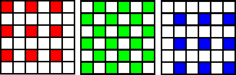
To implement Bayer image interpolation, you should first extract each channel from the raw image. Then, you will have three channels for the image, but each channel of the image has many missing values. The white blocks in the above figure mean missing pixels of each channel. 3/4 of the R and B channels and half of the G channel are missing. So, you should implement interpolation for each image channel.

For border pixels, you can handle it on your own. You can use zero padding, reflect padding, only use three neighboring pixels, …​ whatever you think is right. Just clarify your method in the writeup. i.e., state why you used that method. If your implementation of interpolation is correct in the non-border regions, you can get full credit. FYI, usually, border pixels matter less in a real camera since a few border pixels are unused after Bayer interpolation. (There are some sensors that do not use Bayer, except them.) That’s one reason for the difference in total pixels and effective pixels in a real camera. However, in this homework, your image size should not be changed, and you should think about how you can handle it.

From the given two sets of feature points, find the fundamental matrix using the normalized eight-point algorithm. Use the normalize_points function to normalize points.

We have learned the definition and properties of fundamental matrices. After implementing Bayer image interpolation, you should implement the eight-point algorithm to find the fundamental matrix. Details for the eight-point algorithm is described in the supplementary slides in the provided zip file. You can study only the "Eight Point Algorithm: Implementation" slide to implement this task, but "Eight Point Algorithm: Proof" slides in the supplementary material will be helpful if you are interested in optimization methods and a detailed proof for the normalized eight-point algorithm.

Note that a fundamental matrix can convert an image point into its epipolar line on the opposite image. After implementing calculate_fundamental_matrix, hw3_main.py will generate an image file result/imgs_epipolar_overlay.png, which is overlayed with the feature points and their epipolar lines. You can utilize this image to check your implementation qualitatively.

After finding the fundamental matrix, you should rectify your cameras. It means that we need to reproject the input image planes onto the common plane parallel to the line between camera centers. After the reprojection, the pixel motion will be horizontal. This reprojection is formed as two homography matrices(3*3) \(H\) and \(H'\), one for each input image reprojection. Those \(H\) and \(H'\) can be derived from the fundamental matrix and feature point sets. However, it requires many more steps than we covered in the lecture. Thus, finding \(H\) and \(H'\) is done by the OpenCV native function cv2.stereoRectifyUncalibrated(), and you do not need to work on that part. What you need to do is the following two tasks.

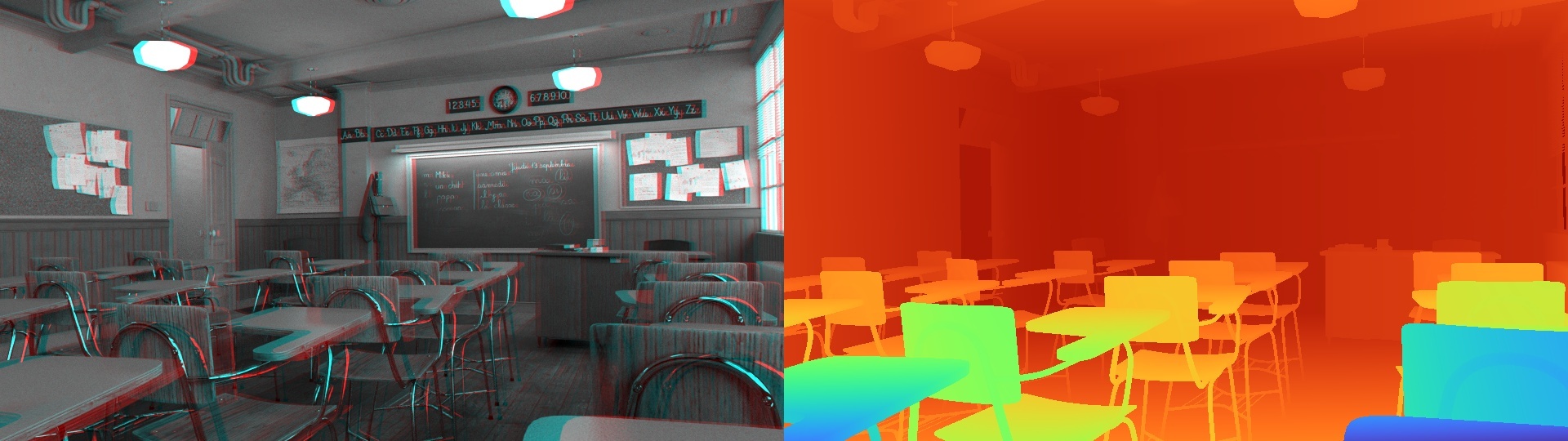
It is possible to estimate a disparity map from your rectified images. But for better evaluation of a disparity map estimation itself, we provide perfect rectified images from a calibrated camera (data/img3.png and data/img4.png) and ground truth disparity map (data/img3_disp.npy). The data reading part has already been implemented, so you don’t need to work on it. And, of course, do NOT utilize ground truth disparity to calculate your disparity map. If we find this kind of cheating, you will get 0 points in this homework, whatever you did.

The final goal of this task is to get the disparity map of first image (left image, data/img3.png). In other words, for such point \((x,y)\) in first image, the corresponding point in second image (right image, data/img4.png) is given as:

where \(\mathbf{d}(x, y)\) is disparity map of first image. (Hint: In general binocular stereo setup and the rectified left/right images, \(\mathbf{d}(x, y)\) of left image might have negative values. i.e., maximum possible disparity is 0. Think why it happens.) Since this process takes a long time, it is recommended to print the progress of computation log to check your code is running (e.g., print iteration numbers, using the tqdm library or any other methods).

Before starting, there are some hyperparameters such as NCC window size, minimum and maximum disparities, and cost aggregation window size. Try various hyperparameter values and search for good values on your own. Provide your findings in the writeup. For the window size parameters, you are allowed assume it will be only the odd numbers.

In addition, you may see some numerical computation warnings for this task, such as zero-division or overflow. Make sure your code does NOT produce such numerical warnings. If your result contains nan (not a number) or inf (infinity), it will be reported as 0 points on the evaluation.

Total 20pts

To get extra credits, you MUST describe BOTH the original version and the extra-credit version in the writeup. For code submission, you can submit only the extra credit-enabled code with parameters to switch between the original task and the extra credit task.